GPT-2 Implementation From Scratch For Dummies!

If you ever had trouble understanding the code behind the attention mechanism and the research paper's complex code, this is for you.

In this post, I break down the inner workings of a GPT-2 model—from token embeddings and positional encodings to multi-head self-attention and MLP blocks. I'll try to "dumb" things down and explain the details and intuition behind each line of code as much as I can. If you're a dummy like me, I hope this helps.

1. Input & Token Embeddings

The input to LLMs is a batch of sequences, so usually the input is a matrix of shape (batch_size B, sequence_length T).

B represents the batch size, T represents the number of tokens in a specific sequence.

2. Token Embedding Layer

First layer is the token embedding layer with the shape of (vocab_size V, hidden_size C):

• vocab_size: Total number of tokens in our vocabulary

• hidden_size or n_embd: number of dimensions we want to embed each token to. For example if hidden_size = 768 then each token would be represented with a vector of 768 entries.

3. Token Embedding Output

After going through the token embedding layer (This operation is not matrix multiplication, it's more of a look up table), the resulting output has the shape (batch_size B, sequence_length T, hidden_size C).

This happens because now we go through the batches, in every batch we have a sequence of tokens with tokens being numbers ranging from 0 to vocab_size - 1 and now we replace each token with a vector of size hidden_size C.

4. Positional Encoding

Next layer is the positional encoding layer with the shape of (sequence_length T, hidden_size C).

This means that each position in the sequence will have an embedding representation to give it meaning.

No need to pass any input through the position embedding, it is used to be added after the input comes out from word token embedding layer.

So now we have a matrix with shape of (batch_size B, sequence_length T, hidden_size C) and for each batch size we add the positional embeddings matrix which is (sequence_length T, hidden_size C).

5. Transformer Blocks

Now this input goes through N number of blocks, each block contains layers that do transformations.

A block structure has the following layers:

- LayerNorm layer 1
- self attention layer
- LayerNorm layer 2
- MLP block

The flow / forward pass of the input matrix (batch_size B, sequence_length T, hidden_size C) is as follows:

The shape of the LayerNorm layer 1 is (hidden_size C), for each batch_size, we apply the layer normalization for each token vector. The output shape remains the same (batch_size B, sequence_length T, hidden_size C).

Attention Block

Attention Block is the following:

- query layer: Linear layer (hidden_size C, hidden_size C)
- key layer: Linear layer (hidden_size C, hidden_size C)
- value layer: Linear layer (hidden_size C, hidden_size C)
- c_proj: Linear layer (hidden_size C, hidden_size C) 
- mask layer: lower triangle 1 matrix (1, 1, sequence length T, sequence_length T)

The flow / forward pass on the input matrix (batch_size B, sequence_length T, hidden_size C) is as follows:

We first create 3 linear layers (matrices) of query, key and value:

• Query matrix: represents the tokens we want to calculate how much other tokens affect

• Key matrix: represents the tokens that affect the query token

• Value matrix: is the actual value of the token

These are the 3 different representations that we want to create from our input matrix (batch_size B, sequence_length T, hidden_size C). Now we want to create multiple heads of attention that look at different parts of hidden_size.

The idea behind this is that if we use one attention head that looks at all the features of token (meaning it's of hidden_size C), it can focus only on one aspect/view and ignore other views of how tokens can relate to each other.

So we create multiple attention heads, each head looks at a subset of the token's features. With these we can capture different relations between tokens and each head can specialize in different types of relationships.

This is why we compute the head size by dividing the hidden size C by the number of heads:

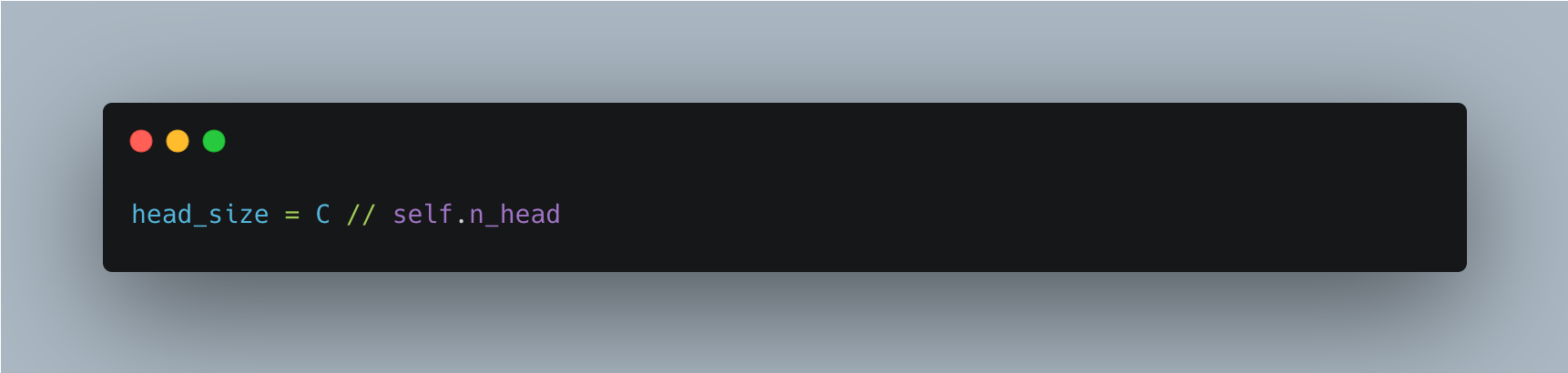
Now we want to reflect that we want multiple heads, each head will look at the sequence T and each sequence has tokens of embedding size head_size hs now:

The result of the view is matrices of size (batch_size B, sequence_length T, number of head nh, head_size hs). We also do a transpose of dimensions 1 and 2 preparing for the matrix multiplication for each head, so that the resulting dimension is (batch_size B, number of head nh, sequence_length T, head_size hd).

Now we compute the attention between different tokens for all the heads:

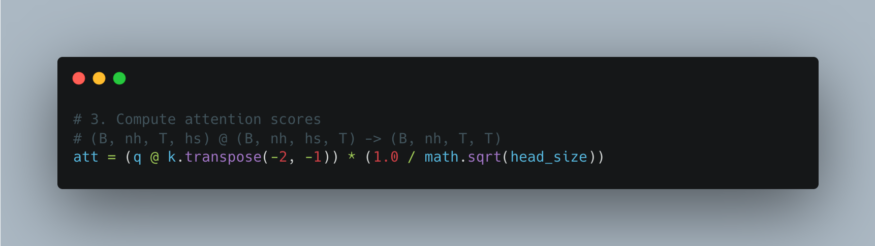
Resulting matrix is of shape (batch_size B, number of heads nh, sequence_length T, sequence_length T). Then we apply the causal mask because we don't want tokens to attend to tokens from the future:

Resulting matrix after masking: (batch_size B, number of heads nh, sequence_length T, sequence_length T).

At this point the numbers don't add up to one and they are raw similarity scores, this is why we want to apply the softmax transformation to put the numbers into a normalized probability distribution. All the values will be between 0 and 1, and the sum across each row (sequence T) will add up to 1.

Resulting matrix after softmax is of shape (batch_size B, number of heads nh, sequence_length T, sequence_length T).

Now we matrix multiply this importance distribution with the actual values matrix:

Resulting matrix after softmax has the shape (batch size B, number of head nh, sequence length T, sequence length T). Then the resulting matrix after value multiplication is (batch_size B, number of head nh, sequence length T, head size hs).

Now that we have the outputs from the attention mechanism from different heads (batch_size B, num_heads nh, sequence_length T, head_size hs), we need to reshape it again to combine the results from different heads. That's why we transpose positions 1 and 2 resulting in a matrix with the following shape (batch_size B, sequence_length T, num_heads nh, head_size hs). Now we combine the results from the different heads ending up with a matrix of size (batch_size B, sequence_length T, hidden_size C).

We then pass it through a linear layer to learn a combined coherent features from the resulting separate features of the attention mechanism coming from different heads.

MLP Block

Now we need to define the MLP block:

- c_fc: Linear layer (hidden_size C, hidden_size C * 4)
- gelu: GeLU activation layer (gelu with tanh activation)
- c_proj: Another Linear layer (hidden_size C * 4, hidden_size C)

The flow or the forward pass of the input matrix (batch_size B, sequence_length T, hidden_size C) through the MLP block is as follows:

The idea behind the first layer c_fc is to project into a higher dimension (from hidden_size C to 4 * hidden_size C) space to learn more features. Then we apply non-linear GELU transformation, it softly gates input values, values closer to zero are shrunk more smoothly rather than being zeroed out.

Second linear layer reduces the dimensionality back to hidden_size C from 4 * hidden_size C so now we end up again with a matrix of shape (batch_size B, sequence_length T, hidden_size C) and this output gets into the next block.

6. Final Layers

After we're done with N blocks, we have two final layers:

- ln_f: Layer norm 
- lm_head: Linear layer (hidden_size C, vocab_size V)

This layer will project the embeddings back to vocab_size, now we have logits for each one of the tokens they are not probabilities just yet (we need to add softmax). We also set this layer with bias=False as biases are unnecessary at this stage and removing them saves memory.

We also introduce the idea of weight sharing / tying which basically consists of making the token embedding layer and the lm_head layer essentially the same.

If we look at matrices shapes, we see that the input embedding layer has shape of (vocab_size V, hidden_size C) but the output projection layer or lm_head has the shape (hidden_size C, vocab_size V). By doing the following weight tying:

We're essentially modifying the pointer for the matrix wte.weight to now point to the same memory address as lm_head.weight. At a first glance I thought this would result in a shape mismatch error when doing the forward pass, but it doesn't happen because nn.Linear layer does the transpose operation behind the scenes.

The intuition behind doing this "weight tying" is that both of these layers go to/from embeddings to/from vocab_size. So they either create embeddings for each token or create logits for each token from the embeddings. The way that tokens are represented internally needs to align with the way the model predicts the tokens. This has many benefits such as you get 1 layer instead of 2 separate layers which means less storage space and more speed.

Forward Pass

This is how the whole forward pass looks like in Python:

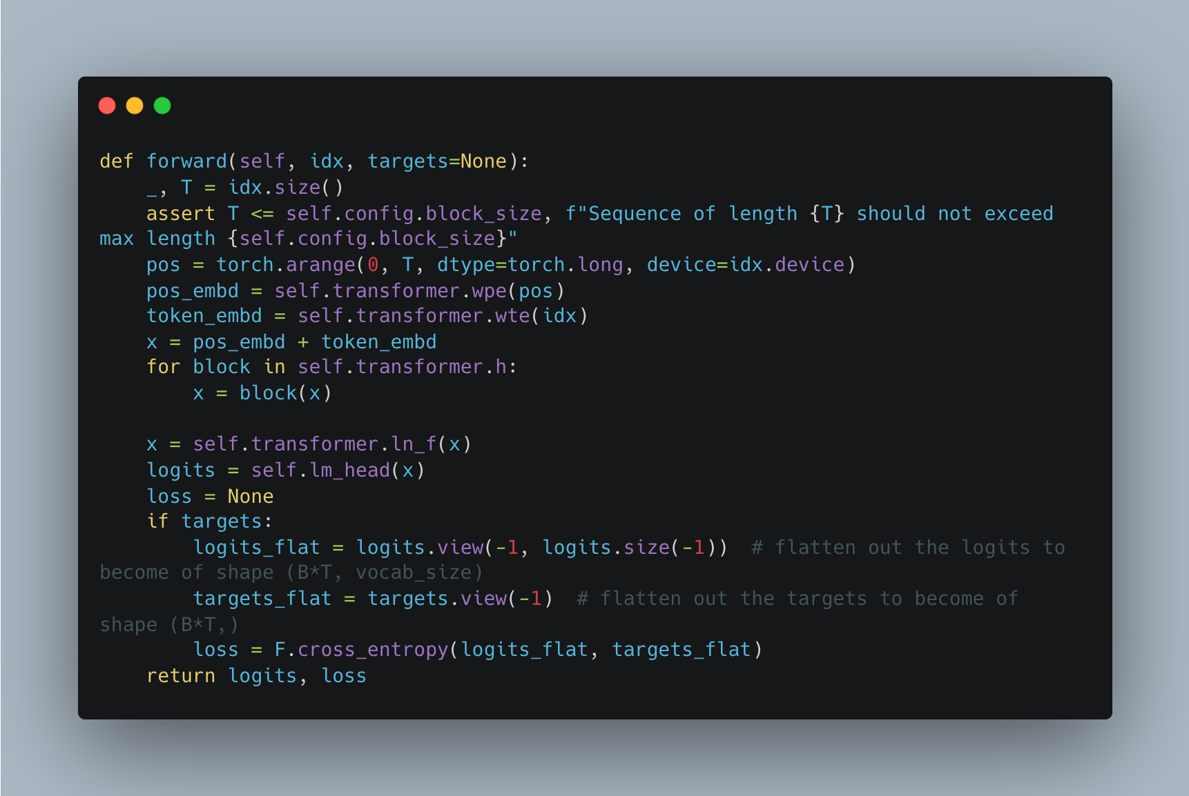
The pos variable coming from the torch tensor torch.arange(0, T, dtype=torch.long, device=idx.device) is basically the PyTorch implementation of list(range(0, T)) so that we have a tensor that contains numbers from 0 to T.

We pass this tensor later on wpe (word position embedding), so that we have an embedding for each position between 0 and T.

We pass the input tensor idx which is of shape (batch_size B, sequence_length T) to wte to create embeddings for each input token and then add them together:

We later have to flatten out the logits which are of shape (batch_size B, sequence_length T, vocab_size V) and the targets (batch_size B, sequence_length T).

PyTorch's F.cross_entropy expects:

• Predictions: (N, C) where N = number of samples, C = number of classes

• Targets: (N,) a 1D tensor of class indices

Then we calculate the cross entropy cross_entropy loss.

Next blog post, we can look at other details such as how to load the data, how to tokenize and how to actually run the training.

References;

• NanoGPT from Andrej Karpathy, https://github.com/karpathy/nanoGPT

• Andrej Karpathy’s YouTube video explanation,

Feel free to clap, follow, and comment if you enjoyed the article!

Stay In touch by connecting via LinkedIn Aziz Belaweid or GitHub.