Your Complete Guide to RCNN, Fast-RCNN, Faster-RCNN and Mask-RCNN
In this article, I provide a detailed overview and summary of the RCNN family.
This article helps you navigate the transition from one architecture to another and explaining the obstacles of each and how these obstacles were solved.
RCNN
Architecture
RCNN uses a region proposal algorithm to extract regions of interest, this proposal algorithm is mainly selective search or bounding box (greedy algorithms that segment ROI then combine them)
Selective search generate about 2000 regions, each of those regions is passed into a CNN ( this can be VGG or AlexNet or any CNN of your choice but mainly VGG is used)
Region proposals are not of the same size that’s why we wrap them into a fixed size region proposal.
The CNN acts as a feature extractor, it’s output is a dense feature vector that’s saved to the disk and then passed to an SVM that will classify the presence of an object within that region.
The feature vector is also fed to a Bounding Box regressor that will fine-tune the region boundaries.
Obstacles
RCNN takes a huge amount of time to classify the 2000 region proposals per image(CNN will do 2000 forward passes per image) making it hard for it to work in real time. Selective Search is a fixed algorithm and not learnable which hinders both speed and accuracy.
RCNN also consumes significant space because it saves the produced feature vector to the disk.
Training takes 84 Hours
Test time 47s per Image using VGG16
Fast-RCNN
Architecture
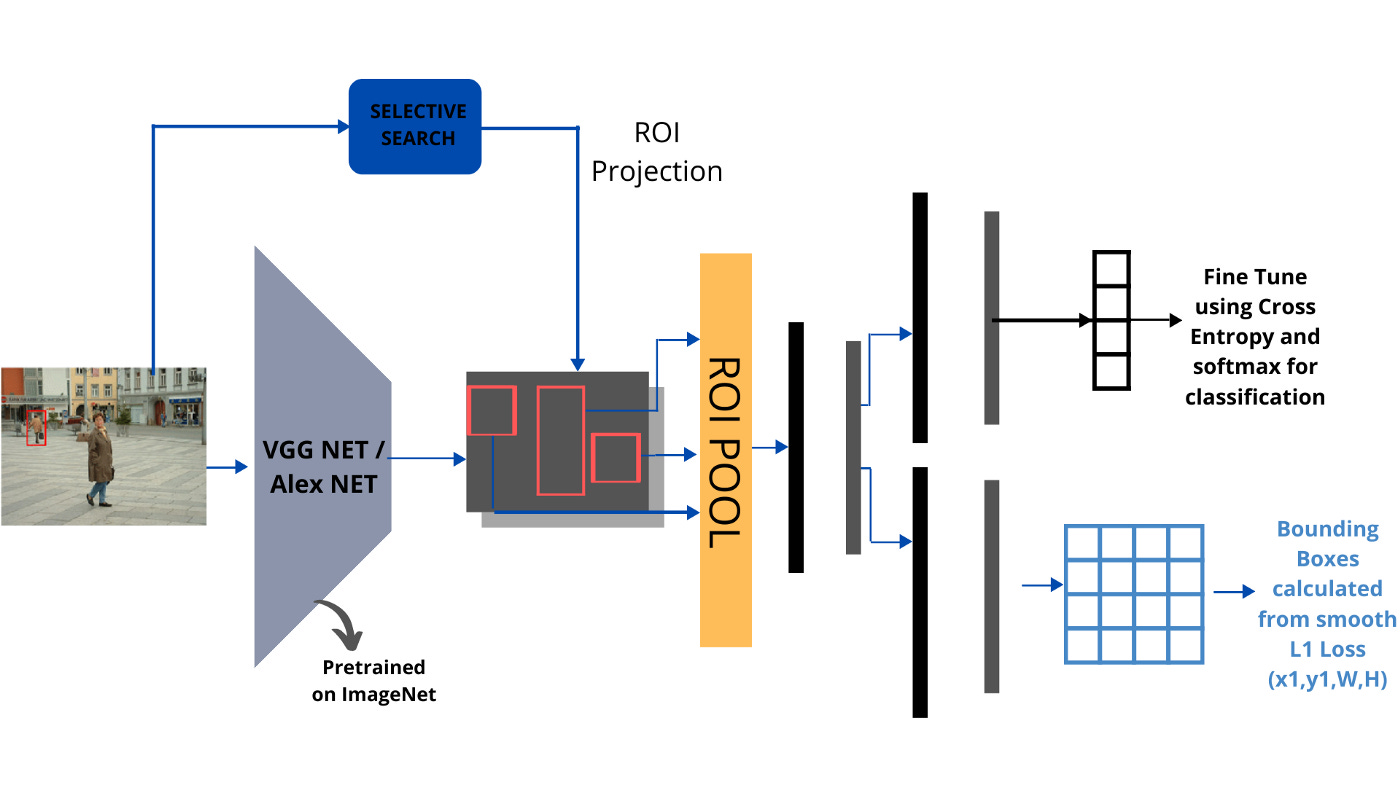
The main idea behind Fast-RCNN is now we would like the CNN to do one forward pass over the image and then project the 2000 extracted regions from selective search onto the feature maps produced by the CNN. This is called ROI projection.
Before this, we must calculate the Subsampling ratio which is the ratio of the final feature map size divided by the original image size.
They also introduce the concept of ROI pooling, this is because the final fully connected layers need a fixed sized input, but we have different sizes of region projections on the feature map so we need a way to make them all the same size.
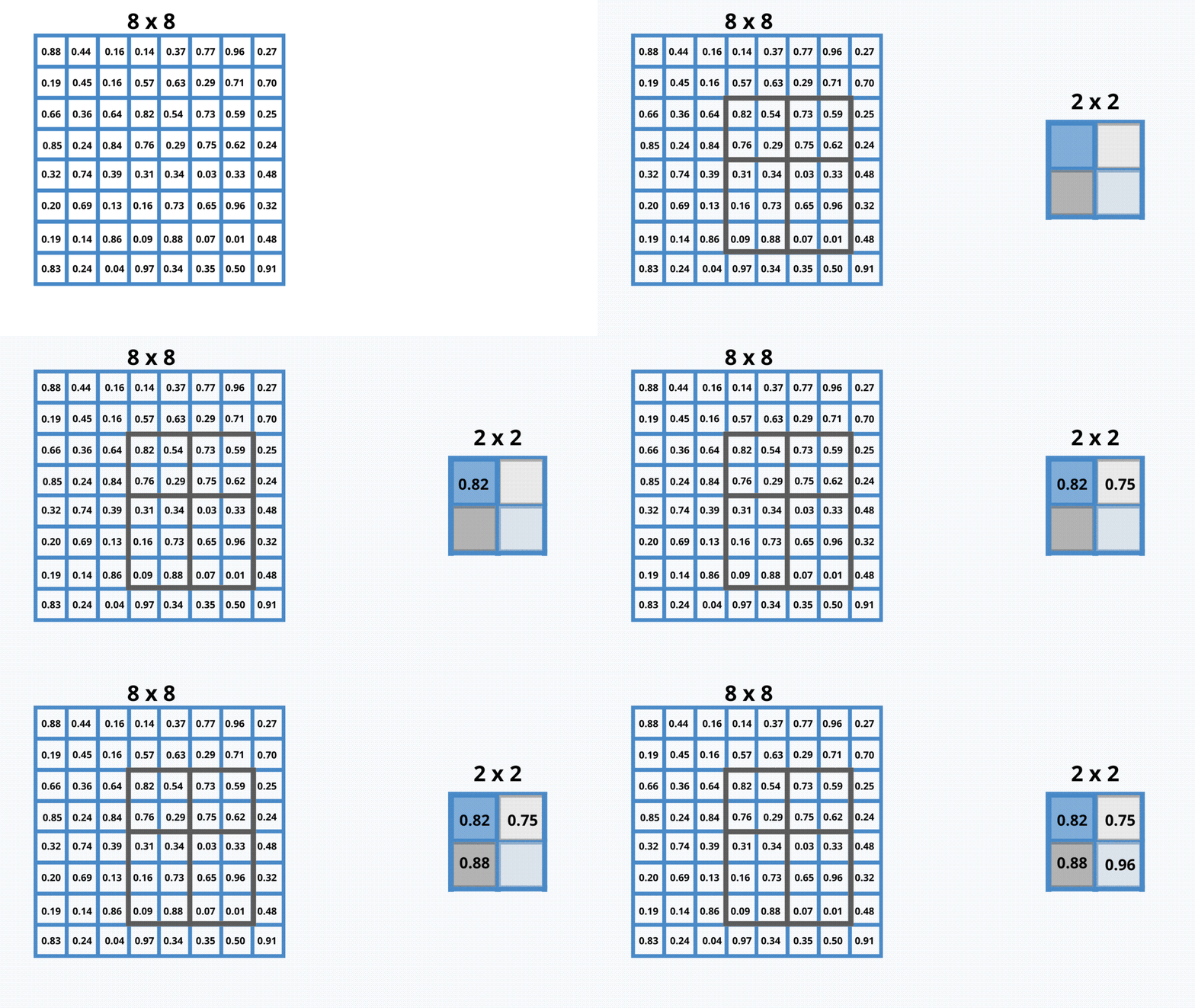
RoI max pooling works by dividing the h × w RoI window into an H × W grid of sub-windows of approximate size h/H × w/W and then max-pooling the values in each sub window into the corresponding output grid cell.
Pooling is applied independently to each feature map channel, as in standard max pooling. The RoI layer is simply the special-case of the spatial pyramid pooling layer used in SPPnets in which there is only one pyramid level.
Here they choose H=W=7
Example:
As shown above, consider the red box as the ROI Projection onto the 8 x 8 feature map. Let’s assume that we need a 2 x 2 dimensioned output. Then dividing them equally may not be possible if there is an odd-numbered dimension. In such cases, we’ll round off to the nearest value. As shown, assume we get a 5 x 4 sized proposal. To convert it into a fixed dimensional box, we divide the height and width to that of the required ones i.e., 5/2 x 4/2 = 2.5 x 2. Rounding it on them, either way gives 2 x 2 and 3 x 2. Then each block is max-pooled and the output is calculated. In this way, we get a fixed dimensional output for any variable-sized region proposal. So now, there’s no restriction on the size of the input.
Fast-RCNN also gets rid of the SVM classifier and replaces it with softmax, also the bounding box regressor now uses L1 loss.
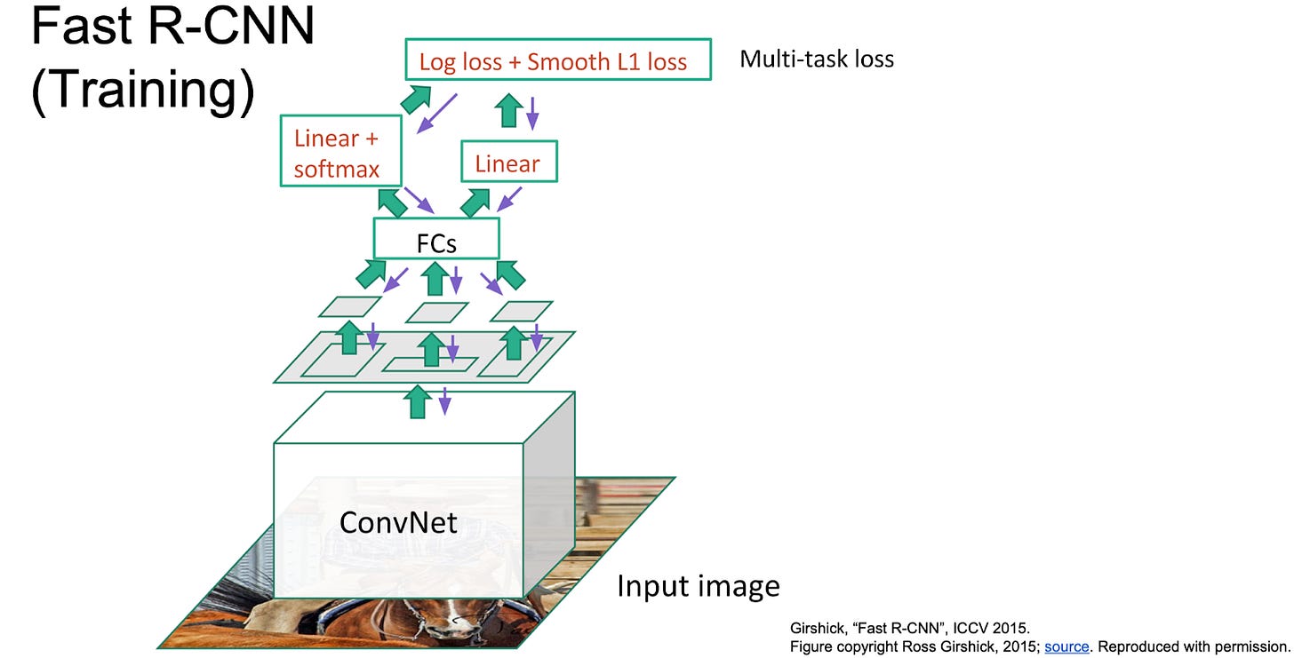
Training is done using backpropagation on multitask loss.
Results
Obstacles
Selective search still represents a bottleneck, it’s not learnable and takes time to produce region proposals.
Faster RCNN
Architecture
Even though with Fast-RCNN we made great improvements over RCNN yet still remains one bottleneck that we need to solve which is Selective Search, we need a solution that proposes less than 2000 regions, faster and as accurate as Selective Search.
Why not use the same CNN results for region proposals ?
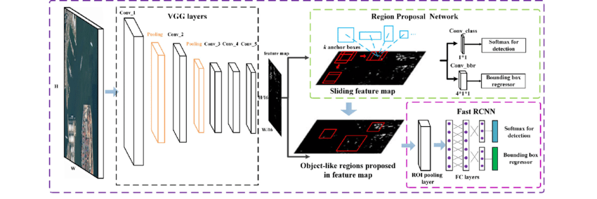
The ultimate goal here is to share computations between region proposals and the rest of the network. We share the convnets then the feature maps are fed into a Region Proposal Network Network (RPN), a sliding window of size 3x3 (this is changeable) is applied. At each sliding-window location we predict multiple proposals using 9 anchor boxes (this is changeable) The anchor boxes are of different sizes and aspects to be able to capture overlapping objects. We place them at the center of the sliding window.
We pass the proposed region into 1x1 conv layers one for regression and one for classification. We use regression to predict the bounding box and we use classification to reduce the number of proposed regions ( background or not)
Non Maximum suppression is also applied to eliminate more proposals. Then we project the proposed regions on feature maps and do ROI pooling the same as Fast-RCNN.
The Faster R-CNN is jointly trained with 4 losses:
RPN classification (Object foreground/background)
RPN regression (Anchor → ROI)
Fast RCNN Classification (object classes).
Fast RCNN Regression (ROI → Bounding Box
Results
Mask RCNN
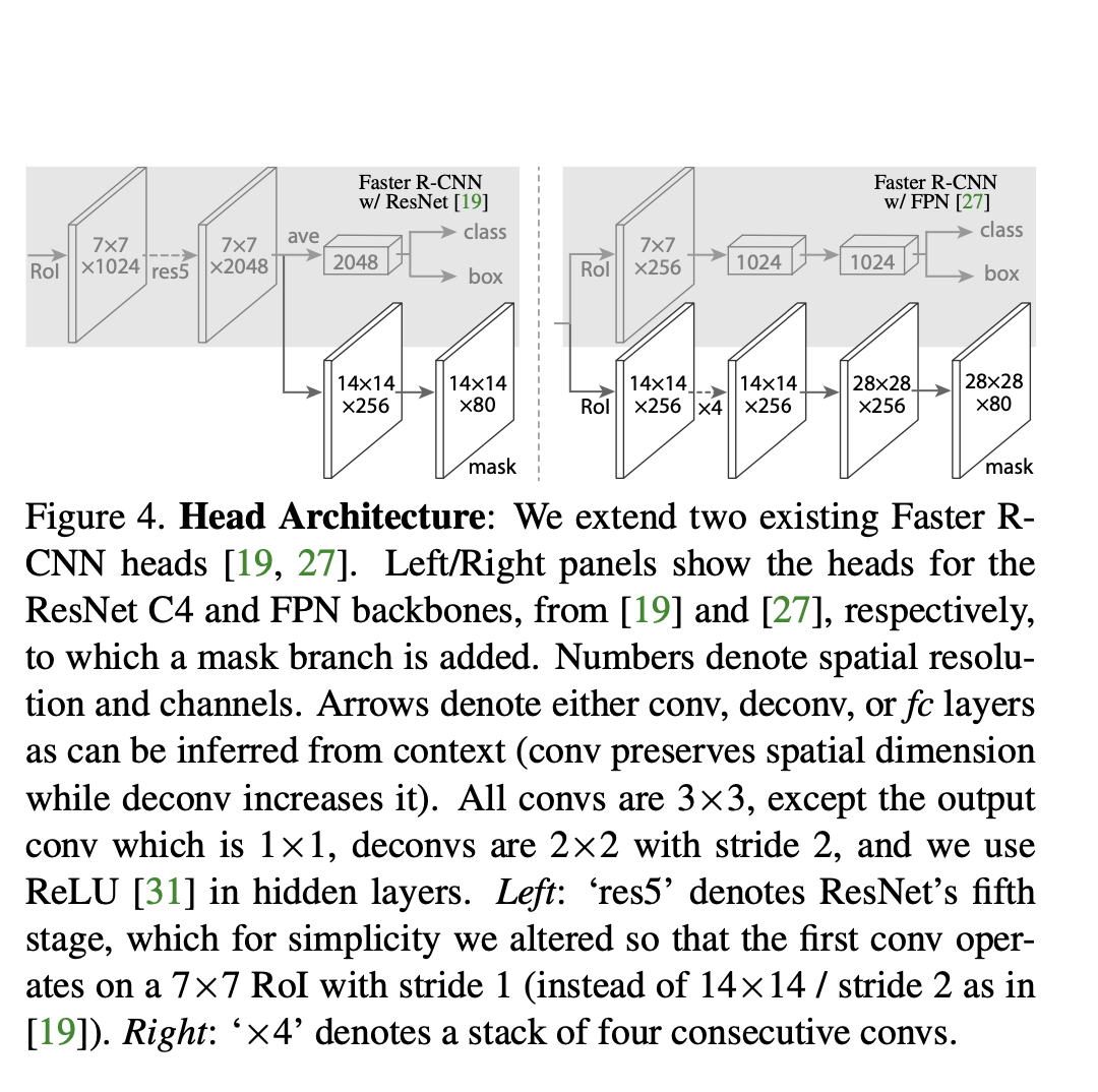
Mask R-CNN, extends Faster R-CNN by adding a branch for predicting an object mask in parallel with the existing branch for bounding box recognition.
Mask R-CNN adopts the same two-stage procedure, with an identical first stage (which is RPN). In the second stage, in parallel to predicting the class and box offset, Mask R-CNN also outputs a binary mask for each RoI.
We define a multi-task loss on each sampled RoI as L = LCls + LBox + LMask.
The mask branch is a small FCN applied to each RoI, predicting a segmentation mask in a pixel-to- pixel manner.
The mask branch predicts a binary mask for each RoI using fully convolutional layers; they use sigmoid instead of softmax activation. The class prediction branch is used for class prediction and for calculating loss, the mask of predicted loss is used in calculating LMask.
Faster R- CNN was not designed for pixel-to-pixel alignment between network inputs and outputs.
For each RoI, RoIPooling first “finds” the features in the feature maps that lie within the RoI’s rectangle. Then it max-pools them to create a fixed size vector.
Problem: The coordinates where an RoI starts and ends may be non-integers. E.g. the top left corner might have coordinates (x=2.5, y=4.7). RoIPooling simply rounds these values to the nearest integers (e.g. (x=2, y=5)). But that can create pooled RoIs that are significantly off, as the feature maps with which RoIPooling works have high (total) stride (e.g. 32 pixels in standard ResNets). So being just one cell off can easily lead to being 32 pixels off on the input image.
For classification, being some pixels off is usually not that bad. For masks however it can significantly worsen the results, as these have to be pixel-accurate.
In RoIAlign this is compensated by not rounding the coordinates and instead using bilinear interpolation to interpolate between the feature map’s cells.
Each RoI is pooled by RoIAlign to a fixed size feature map of size (H, W, F), with H and W usually being 7 or 14. (It can also generate different sizes, e.g. 7x7xF for classification and more accurate 14x14xF for masks.)
If H and W are 7, this leads to 49 cells within each plane of the pooled feature maps.
Each cell again is a rectangle — similar to the RoIs — and pooled with bilinear interpolation. More exactly, each cell is split up into four sub-cells (top left, top right, bottom right, bottom left). Each of these sub-cells is pooled via bilinear interpolation, leading to four values per cell. The final cell value is then computed using either an average or a maximum over the four sub-values.
Their backbone networks are either ResNet or ResNeXt (in the 50 or 102 layer variations).
Their head is either the fourth/fifth module from ResNet/ResNeXt (called C4 (fourth) or C5 (fifth)) or they use the second half from the FPN network (called FPN).
They denote their networks via backbone-head, i.e. ResNet-101-FPN means that their backbone is ResNet-101 and their head is FPN.
Clap, Follow and Comment if you like the article!
Stay In touch by connecting via LinkedIn Aziz Belaweid or GitHub.


